Solving Threes
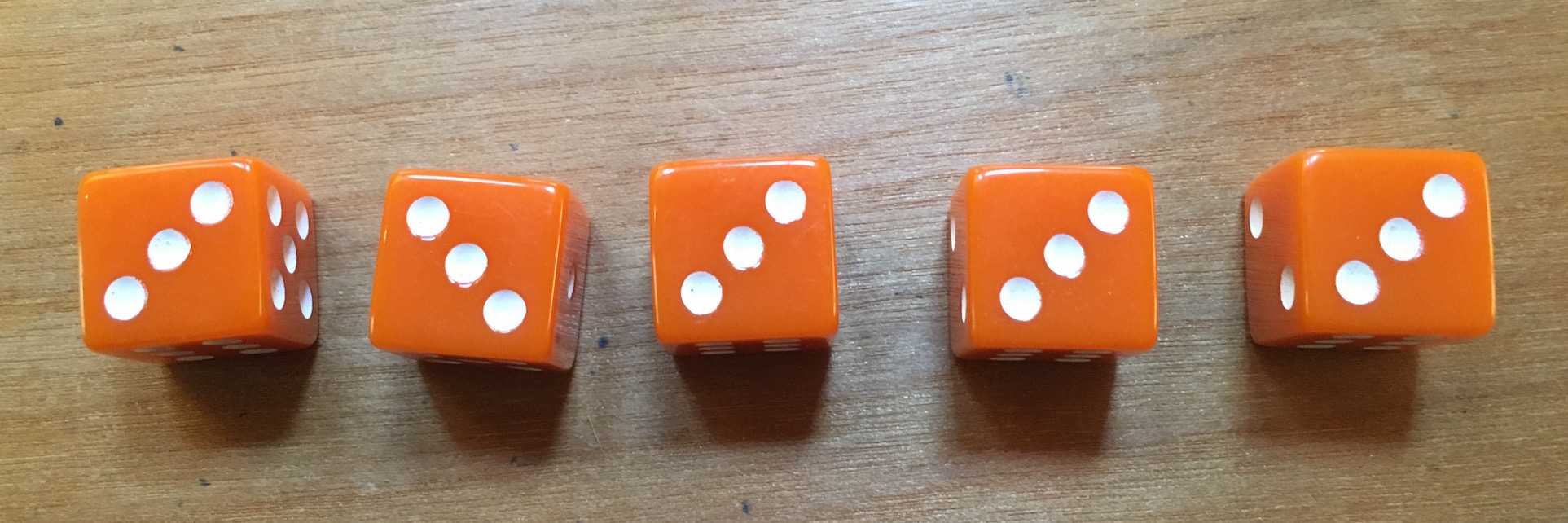
All threes—the infamous hallelujah roll.
Threes: How to Play
Threes is a dice game played by two or more people. The goal is to roll the dice and collect the lowest numbers, where three counts as zero. You’re supposed to take at least one dice per roll, but if you roll all high numbers (like all fives and sixes) you can choose to re-roll them with the consequence of taking at least two dice on the next roll. You can’t accumulate re-rolls (for example by take no-dice multiple times), and you can’t re-roll the last die—you have to take it. An example game is at the bottom of the page.
Backward Induction
To find the optimal policy I’m going to use backward induction. Backward induction works by finding the optimal action at the last step of the game and uses it to find the optimal action at the second to last step, continuing all the way to the current step.
To avoid stepping backwards in time at every roll, we compute a so-called value function containing numbers that determine the optimal action at a given point in the game. The bulk of the challenge in backward induction is computing the value function. Before doing this, we need to set up the game representation and notation.
Game Representation
The game has three main components:
-
States: Game states consist of a list of rolled dice values and a binary take-two indicator. For example, the state \(s = ((0,2,4,6),T)\) indicates a roll of \((0,2,4,6)\) with take-two set to True. The value \(3\) is written as \(0\) and the other outcomes are written in sorted order. Sorting is done because we’re going to refer to dice using an index and we want low indices to correspond to low dice values.
-
Actions: An action is an integer \(a\) indicating the number of dice to take. Since we’re trying to minimize score, we’ll assume that these are the lowest \(a\) dice. Note that \(0 \le a \le len(r)\), where \(r\) is the roll-list.
-
Dynamics: Dynamics are determined by a pseudo-random number generator that gives each dice a uniformly random outcome. Agent actions are determined by a policy \(a(s)\) that maps states to actions. Note that an agent is fully specified by its policy and in this sense the agent is its policy.
Rolling First
If you roll first, you don’t know what your opponent’s score will be, so your best bet is to minimize your final score.
To find the policy that does this, we’ll make a probabilistic model of the dice outcomes and use it to predict which actions will result in which scores, then we’ll choose the action that minimizes expected score.
In the parlance of backward induction we’re treating the game as a Markov decision process and we’re solving it using backward induction on the Bellman equation. Here’s an example to simplify:
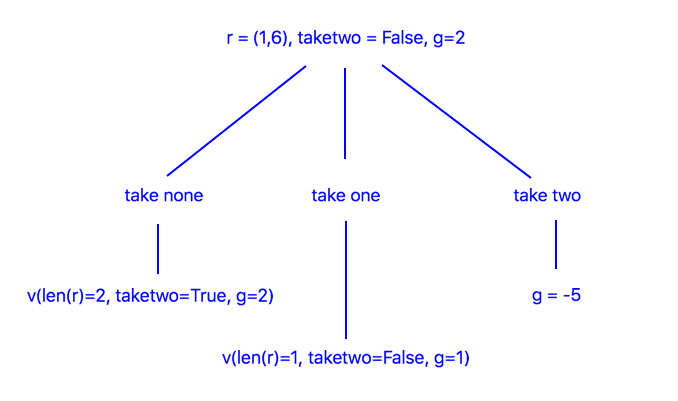
Suppose there are two dice left and we don’t have to take two and we roll \((1,6)\). The diagram below shows the decisions we can make.
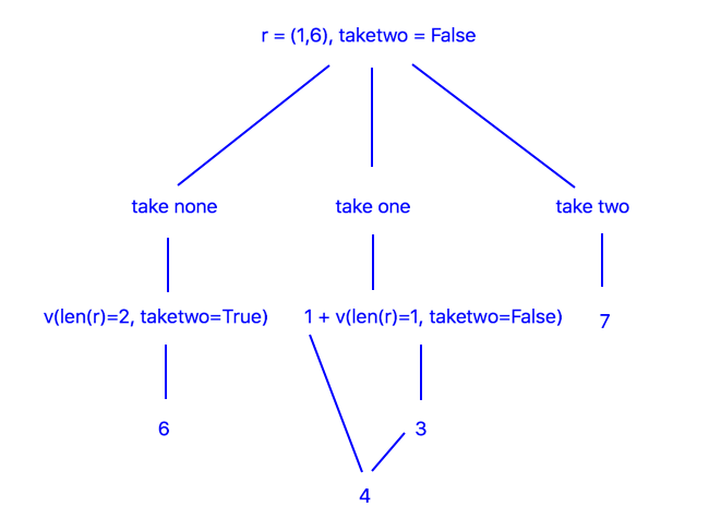
The quantity \(v\) indicates how many points we expect to collect on the next roll, assuming we select the corresponding action. For example, \(v(len(r)=2,\texttt{taketwo}=T) = 6\) because rolling two dice and collecting them both gives a total of \(6\) on average. The bottom of the tree contains numbers that are used to make our final decision. In this case \(a=1\) is the optimal decision because cost plus value is minimum.
One more example, then we can generalize the solution:
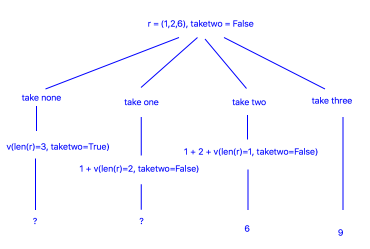
In this case we can’t choose an action because we don’t know \(v(len(r)=3, \texttt{taketwo}=T)\) or \(v(len(r)=2, \texttt{taketwo}=F)\), but we can approximate them using simulations. For example, \(len(r)=2, \texttt{taketwo}=F\) is the situation shown in the first tree, and we were able to make a decision there, so we’ll simulate this situation several times and average the score of the optimal action there. The result is \(v(len(r)=3, \texttt{taketwo}=T)=7\). Using a similar technique we find that \(v(len(r)=2, \texttt{taketwo}=F)=4\).
Thus the optimal action is \(a=1\). Notice that we had to simulate backward starting from the end of the game. This is the defining property of backward induction. To prevent redundant simulations, we cache values so we only have to simulate once per state, afterwards we can just look-up the information we no to act.
The Value Function. Once we have all the values \(v\) it’s simple to choose the optimal action from an arbitrary state: choose the action that minimizes immediate points plus next-state value. Notice that \(v\) depends on the number of dice being rolled and the dice values themselves. This means the game can be represented more simply in terms of the number of dice rolled \(len(r)\) and the take-two indicator. The values are organized in a table called the value function. Here it is:
| len(r) | taketwo | v |
|---|---|---|
| 1 | F | 3 |
| 2 | T | 6 |
| 2 | F | 4 |
| 3 | T | 7 |
| 3 | F | 4.8 |
| 4 | T | 7 |
| 4 | F | 5.3 |
| 5 | T | 7 |
| 5 | F | 5.6 |
The Optimal Policy. The value function together with the heuristic “choose the action which minimizes immediate points plus next-state value” defines the optimal policy. Here’s the corresponding formula:
Where \(r[0:a']\) is the number of points gained from the immediate action, and \(v(len(r)-a',a'==0)\) is the value of the next state assuming action \(a'\) is taken.
Experiments. Let’s do some experiments to see how well the optimal policy does. Here’s a comparison between the optimal policy and a policy that takes one lowest dice on every roll, the “playing it safe” policy. 30,000 games were simulated:
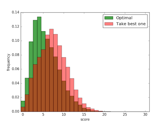
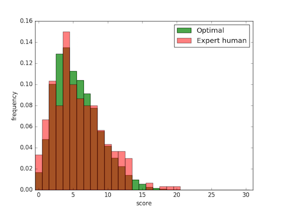
Here’s a comparison between the optimal policy and my policy. To approximate my policy I played Threes three hundred times and recorded my score after each game (yes I actually did that). On average the optimal policy gets a score of 5.6, while I get a score of 5.8. Evidently I play approximately optimally, but I already had the feeling I did :).
Rolling Second
If you roll second you know what score to beat, so instead of acting to minimizing final score it’s best to maximize probability of winning, i.e., get a score lower than your opponent. Again it’s helpful to start with an example.
Suppose you roll two dice, resulting in \((1,6)\), and the opponent’s score is \(5\) and your score-so-far is \(3\), and you don’t have to take two. We’ll parameterize the problem in terms of the gap \(g\) between your score and the opponent’s. In order to win or tie you need \(g \ge 0\). In this example \(g=2\). This decision tree shows the available actions:
The values, i.e., the probabilities of winning, are computed by simulation. For \(a=0\) we simulate collecting two dice, and for \(a=1\) we simulate taking one dice with an update to \(g\) to account for the dice we took. The results are
and
Thus we choose \(a=1\). Note we didn’t consider \(a=2\) because it makes \(g < 0\).
The Value Function. The value function is a little more complicated compared to when rolling first; it now depends on \(g\), which can have up to 30 values. Instead of listing all the values in a table, I’ll put them in a code snippet that includes how they’re computed.
# adjust these as needed
taketwo = False
nleft = 5    # referred to as "len(r)" in the post

d = [0,1,2,4,5,6] # possible dice values

def get_pwin(nleft,taketwo,g):
    # return the probability of winning for the given input state.  these are the values of the value function.
    if (nleft, taketwo) == (1, False):
        return [0.1667, 0.3334, 0.5001, 0.5001, 0.6668, 0.8335, 1.000][g]
    elif (nleft, taketwo) == (2, True):
        return [0.028, 0.083, 0.166, 0.221, 0.304, 0.414, 0.581, 0.691, 0.774, 0.829, 0.912, 0.967, 0.995][g]
    elif (nleft, taketwo) == (2, False):
        return [0.093, 0.238, 0.398, 0.508, 0.623, 0.724, 0.849, 0.914, 0.950, 0.972, 0.993, 0.999, 0.999][g]
    elif (nleft, taketwo) == (3, True):
        return [0.0162, 0.0582, 0.1297, 0.2077, 0.2954, 0.3857, 0.4987, 0.5955, 0.6814, 0.7531, 0.8300, 0.8882, 0.9293, 0.9550, 0.9753, 0.9884, 0.9962, 0.9993][g]
    elif (nleft, taketwo) == (3, False):
        return [0.0580, 0.1634, 0.3050, 0.4322, 0.5596, 0.6698, 0.7774, 0.8611, 0.9183, 0.9492, 0.9722, 0.9857, 0.9929, 0.9964, 0.9988, 0.9997, 1.0000, 1.0000][g]
    elif (nleft, taketwo) == (4, True):
        return [0.0142, 0.0528, 0.1237, 0.2125, 0.3125, 0.4161, 0.5249, 0.6290, 0.7208, 0.7944, 0.8556, 0.9016, 0.9357, 0.9587, 0.9752, 0.9859, 0.9928, 0.9964, 0.9983, 0.9993, 0.9998, 1.0000, 1.0000, 1.0000][g]
    elif (nleft, taketwo) == (4, False):
        return [0.0433, 0.1258, 0.2489, 0.3750, 0.4999, 0.6184, 0.7311, 0.8227, 0.8915, 0.9358, 0.9634, 0.9801, 0.9898, 0.9948, 0.9975, 0.9988, 0.9995, 0.9998, 0.9999, 1.0000, 1.0000, 1.0000, 1.0000, 1.0000][g]
    elif (nleft, taketwo) == (5, True):
        return [0.0130, 0.0493, 0.1162, 0.2048, 0.3101, 0.4198, 0.5318, 0.6364, 0.7305, 0.8070, 0.8659, 0.9097, 0.9418, 0.9631, 0.9775, 0.9867, 0.9926, 0.9959, 0.9978, 0.9989, 0.9995, 0.9998, 0.9999, 1.0000, 1.0000, 1.0000, 1.0000, 1.0000, 1.0000, 1.0000][g]
    elif (nleft, taketwo) == (5, False):
        return [0.0356, 0.1059, 0.2144, 0.3359, 0.4604, 0.5793, 0.6940, 0.7910, 0.8659, 0.9190, 0.9535, 0.9746, 0.9868, 0.9934, 0.9968, 0.9985, 0.9993, 0.9997, 0.9999, 0.9999, 1.0000, 1.0000, 1.0000, 1.0000, 1.0000, 1.0000, 1.0000, 1.0000, 1.0000, 1.0000][g]

# approximate the win-probabilities by simulating all actions for all gaps.  this block is fairly dense...
n_sims = 300000
avgs = []
for g in range(nleft*6):
    pmaxs = []
    print('gap = '+str(g))
    for i in range(n_sims):
        r = np.sort(np.random.choice(d,nleft))
        probs = [0 for _ in range(nleft+1)]
        for a in range(nleft,-1,-1):
            if a < 2 and taketwo: continue
            gnew = g-np.sum(r[0:a])
            if gnew < 0: continue
            if a == nleft:
                probs[a] = 1.0
                break
            else:
                probs[a] = get_pwin(nleft-a,a==0,gnew)
        pmaxs.append(np.max(probs))
    avgs.append(np.mean(pmaxs))

print(avgs)   # the average probabilities of winning
The Optimal Policy. The optimal policy for rolling second is:
Here \(v\) is the value/win-probability of the corresponding state-triple; values are listed in the code-snippet above. To evaluate this equation it’s necessary to know the values for all actions being considered.
Initially values are only available for states at the end of the game, so it’s necessary to simulate backward from \(len(r)=1\) to \(len(r)=5\) and place win-probabilities in the value function as they’re discovered. This is the backward part of backward induction.
Experiments. To conclude the study, I’ll roll first against the AI and see how often I win. Here’s the result:
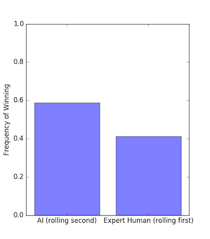
Evidently the AI has an advantage, but it’s probably minimal enough to keep the game fun!
Appendix
Example Game. Here’s an example game, the winner is Player 2 who used a re-roll on the second roll.
Player 1
| Rolled | Collected | Cumulative Collected | Cumulative Score |
|---|---|---|---|
| 4,3,5,3,1 | 3,3 | 3,3 | 0 |
| 4,3,1 | 3,1 | 3,3,3,1 | 1 |
| 6 | 6 | 3,3,3,1,6 | 7 |
Player 2
| Rolled | Collected | Cumulative Collected | Cumulative Score |
|---|---|---|---|
| 3,3,1,2,5 | 3,3 | 3,3 | 0 |
| 6,4,5 | — | 3,3 | 0 |
| 4,4,3 | 4,3 | 3,3,4,3 | 4 |
| 2 | 2 | 3,3,4,3,2 | 6 |
More questions
- Is Threes tractable when the number of dice is much larger than 5, say 5000?
- How would Threes be solved if it had more than two players?