Discovering Class-Hierarchies by Clustering Confusion Matrices
Grouping similar classes into course-grained macro-classes can expose the hierarchical structure of a dataset and guide the development of hierarchical models, but what’s an appropriate way to group classes together? If we interpret a confusion matrix as a similarity matrix, then we can apply clustering on it and the resulting clusters will define the desired macro-classes. In this post I explain this process in the context of a text classification problem.
The Dataset
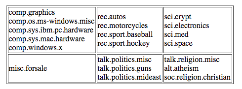
The dataset we’ll use is the classic 20 Newsgroups dataset. 20 Newsgroups contains about 20,000 text documents labelled according to which online newsgroup they were posted in. The different newsgroups/classes are shown below (more info here). The basic problem is to infer a document’s class given only its text.
The Model
To predict document classes, we’ll use a multinomial naive Bayes model applied to tf-idf features. Multinomial naive Bayes (MNB) treats each document as a bag of words that’s sampled from a multinomial distribution. To predict the class of a testing document, MNB computes the log-likelihood of each class given the document’s words and assigns the document to the most likely class: \(c(d)=\arg\max_{c}\log{P(d \vert c)}\).
The multinomial assumption comes into play when we substitute \(\prod_i \theta_{i \vert c}^{n_{i}}\) for \(P(d \vert c)\), producing the classification function
\[c(d)=\arg\max_{c} \sum_i d_{i} \log \theta_{i \vert c}\]\(d_i\) is the number of times word \(i\) appears in test document \(d\) and the \(\theta\)s are probability parameters determined by the words in the training corpus.
Probability parameters are usually set equal to the corresponding word-frequencies, but Rennie et al found that doing so creates unrealistic word-distributions, so to fix this word-counts are commonly transformed into tf-idf features that capture some discriminative properties of real documents.
The tf-idf features are easily computed using scikit-learn’s TfidfTransformer class. This class takes a sparse-matrix of word-counts as input and returns a tf-idf matrix as output, with row \(d\) column \(i\) given by
The denominator of the log counts the number of times word \(i\) appears in other documents. These features can be normalized in various ways. The default normalization in scikit-learn is L2, so each row of the tf-idf matrix is divided by it’s euclidean norm.
The final step is to convert tf-idf values into \(\theta\)s. This is accomplished by normalizing the tf-idf values with respect to class:
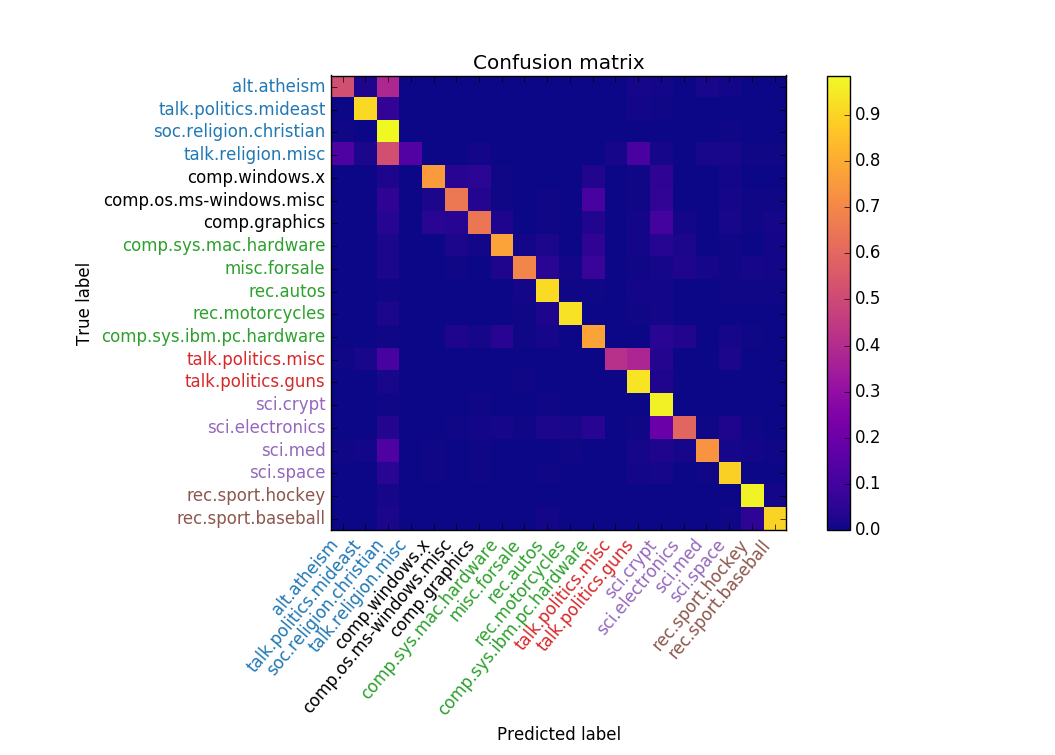
\[\theta_{i|c}=\frac{\sum_{d \in c}{\text{tf-idf}(d,i)}}{\sum_{d \in c,i}\text{tf-idf}(d,i)}\]Now that the features have been transformed and the parameters have been computed, we run the MNB classifier on the 20 Newsgroups dataset and get the following confusion matrix:
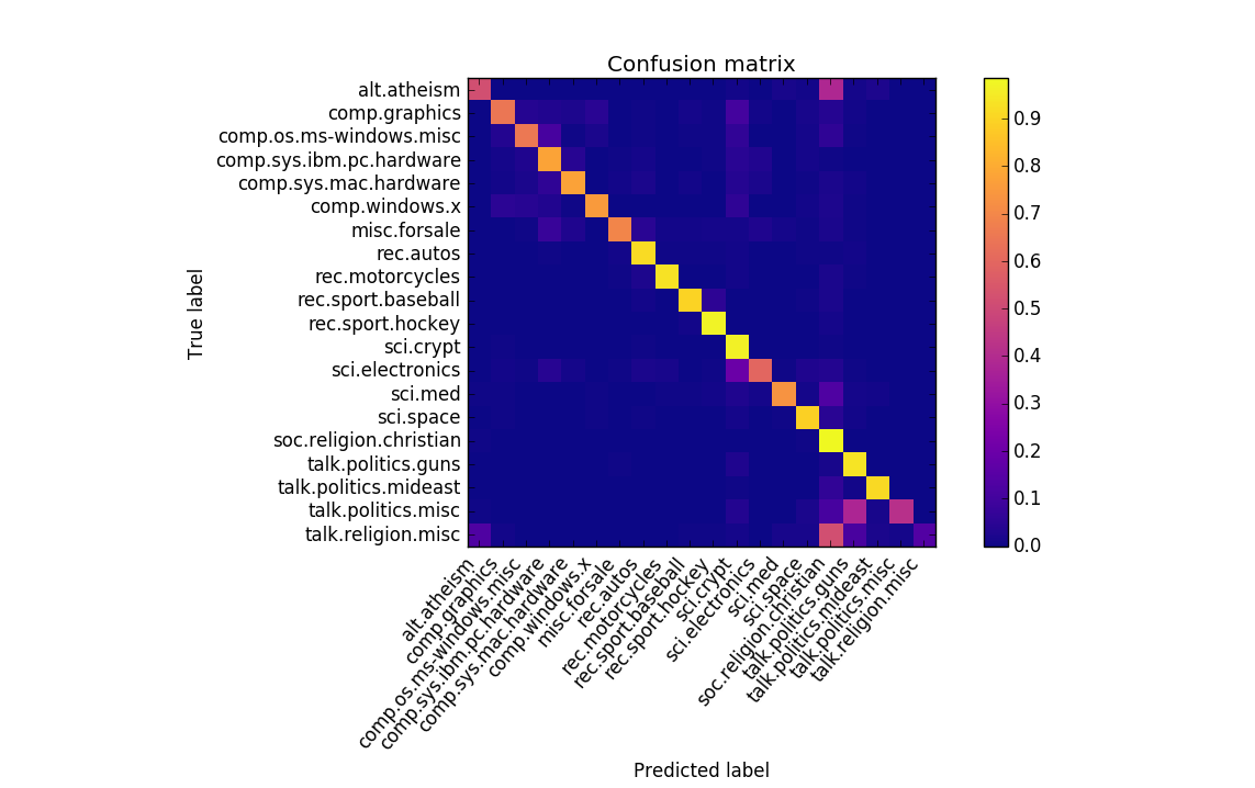
The accuracy is pretty good, but we’re not very interested in accuracy. We’re interested in identifying similar classes that belong in macro-classes together. Such groupings can be done in various ways, but in this post we demonstrate how to do it with a confusion matrix. Grouping via a confusion matrix is nice because all classifiers ultimately generate a confusion matrix, so this technique can be applied to all classifiers, not just ones that have specific feature representations.
Clustering the Confusion Matrix
The key to identifying macro-classes is to interpret the confusion matrix as a similarity matrix and apply clustering on it. A good algorithm for doing this is spectral clustering.
Spectal clustering proceeds as follows (more info here):
- Compute the adjacency matrix \(W\) by symmeterizing the confusion matrix \(W=(C+C^T)/2\).
- Compute the diagonal degree-matrix \(D\) having entries \(d_{ii}=\sum_j{w_{ij}}\).
- Compute the laplacian \(L=D-W\).
- Compute the biggest \(k\) eigenvalues of the laplacian and place the corresponding eigenvectors in the columns of a matrix \(U\).
- Apply \(k\)-means clustering to the rows of \(U\).
The output of this procedure is a set of class indices and their corresponding clusters, which are the macro-class assignments.
To implement spectral clustering, we use scikit-learn’s SpectralClustering class. As with most clustering algorithms SpectralClustering requires the number of clusters \(k\) as an input.
To decide an appropriate value for \(k\) we’ll loop over several values and compute the ratio of intra-class confusion to inter-class confusion for each value. Good clusterings will have high ratios. The results are shown below. We’ve run several trials for each \(k\) (because \(k\)-means is stochastic) and then drawn the average in red.
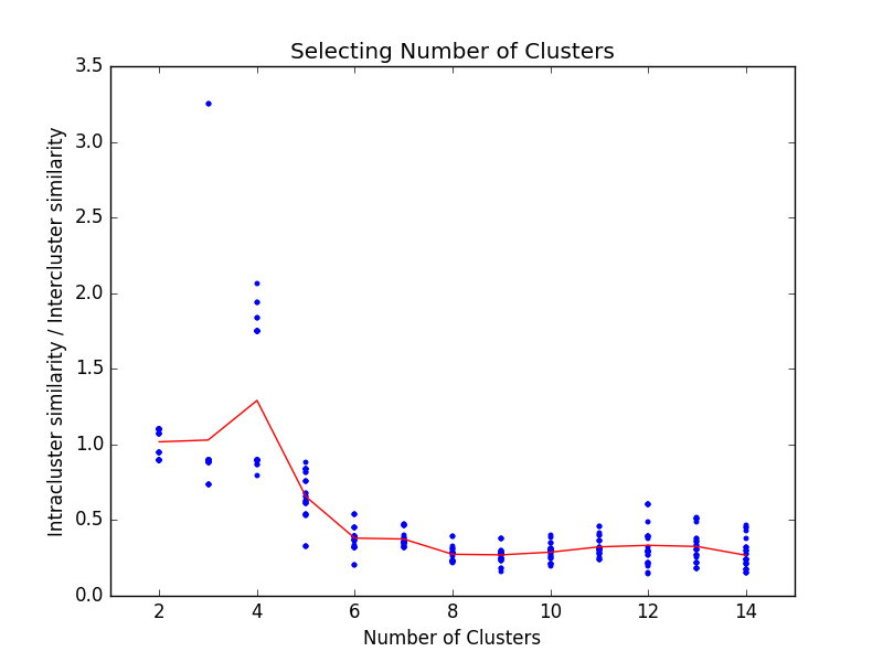
We see that the best clustering occurs when \(k=4\). To visualize the clusters, we re-organize the confusion matrix so classes of the same macro-class are adjacent. The result is shown below.
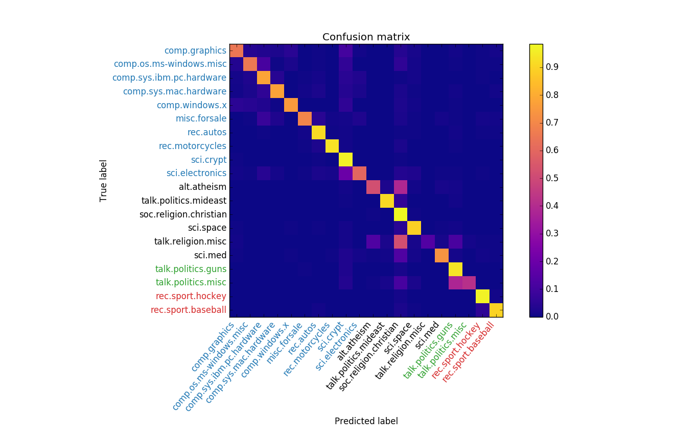
Ideally the confusion matrix will have nice blocks along the diagonal indicating tight clusters, but that doesn’t really happen in this example. Regardless, we see that macro-classes having intuitively similar members are discovered. For example, sports are in a cluster together and so are computer related topics. Setting \(k=6\) as-per the table partitions above gives another reasonable clustering, shown below.
Take-aways
- Confusion matrices can be used to identify macro-classes in a feature-agnostic way.
- Spectral clustering is a good algorithm to do this with.
- Intra-to-inter class confusion is a good metric for identifying \(k\).
- Confusion matrices look good with the
plasmacolor-map inmatplotlib:)