Quantum Mechanics Part I: States & Principles
Systems and Experiments
One way to approach quantum mechanics is by comparing it to classical mechanics through a thought experiment. The experiment involves measuring the spin of a particle using an apparatus that can be oriented in an arbitrary direction. The goal is to develop a mathematical model that captures the relationship between the spin of the particle, the orientation of the apparatus and the measurement value.
For the classical system, suppose we orient the apparatus in the \(+z\) direction, measure the spin, and find it to be \(+1\). Next, we orient the apparatus in the \(-z\) direction, measure the spin, and find it to be \(-1\). Next, orient in the \(+x\) direction and measure \(0\). After more configurations and measurements we find that spin can be modeled as a unit vector \(\hat{\sigma}\) oriented in 3-space relative to the apparatus direction \(\hat{a}\), and the measurement we get is \(\hat{a} \cdot \hat{\sigma}\). Note we’ve assumed that spin is unaffected by measurements—spin is a physical state existing independent of the apparatus and measurements leave it unchanged. As we’ll see this is not necessarily true in QM.
Now let’s do the same experiment on quantum spin. Measuring \(\pm z\) we get the same results as before. But when we measure \(x\), instead of \(0\) we get \(+1\). If we re-run the experiment from scratch and measure \(x\) again, this time we get \(-1\). Repeating many times, the \(x\) measurement returns \(+1\) or \(-1\) in seemingly random order — never \(0\), and never any other value. After taking more measurements a pattern emerges: the quantum result is the same as the classical result but only on average. In other words \(\left< \sigma \right> = \hat{a} \cdot \hat{\sigma}\).
So two things change between CM and QM: outcomes become non-deterministic, and the set of possible outcomes shrinks from a continuum (any value in \([-1,+1]\)) to two discrete values (\(\pm 1\)). Also, classical states are unchanged by measurements. For example, measuring along \(z\) and then \(x\) and then \(z\) returns the original measurement of \(z\). In other words measuring \(x\) doesn’t affect the outcome of \(z\). In quantum mechanics this isn’t always true. The intermediate measurement of \(x\) changes the system such that re-measuring \(z\) may not return the original result.
States
Quantum states are modeled as vectors in so-called Hilbert space. In Hilbert space vectors can be real or complex and have finite or infinite dimension. An example of a finite-dimensional vector is a simple column-vector, and an example of an infinite-dimensional vector is a continuous-valued function (more on those later).
In terms of notation, vectors are drawn as kets \(\ket{\psi}\) that have Hermitian conjugates called bras, drawn the other way around \(\ket{\psi}^{*} = \bra{\psi}\). The inner product of two vectors \(\bk{\psi}{\phi}\) is conjugate-symmetric: \(\bk{\psi}{\phi}^* = \bk{\phi}{\psi}\). Two vectors are orthogonal when \(\bk{\psi}{\phi} = 0\), and a vector is unit-normalized when \(\bk{\psi}{\psi} = 1\). The familiar properties of commutativity, associativity, distributivity and closedness are required in order for kets to be considered proper Hilbert vectors.
A general quantum state can simply be denoted by \(\ket{\psi}\), but it’s often useful to represent it explicitly with components:
\[\ket{\psi} = \sum_i^N a_i \ket{i}\]For now we’ll assume \(N \ne \infty\), meaning this is a finite dimensional vector. The set of \(\ket{i}\) form an orthonormal basis and the set of \(a_i\) are complex components. Note that this representation of \(\ket{\psi}\) implies using a specific basis, and the values of \(a_i\) depend on the basis.
Spin States
How is spin represented in this notation? Let \(\ket{+z}\) and \(\ket{-z}\) be orthonormal bases for the \(z\) measurement such that an arbitrary state prior to measurement is written as
\[\ket{\psi} = a_+ \ket{+z} + a_- \ket{-z}\]Defining the bases as orthonormal is important because it encodes the fact that they are distinct: measuring \(z\) returns \(\ket{+z}\) or \(\ket{-z}\) but never both.
When the values of \(a_+\) and \(a_-\) are squared and normalized they represent measurement probabilities. In other words, \(a_+^{*}a_+\) is the probability of measuring \(\sigma_z = +1\) and preparing \(\ket{+z}\), while \(a_-^{*} a_-\) is the probability of measuring \(\sigma_z = -1\) and preparing \(\ket{-z}\). The probabilities normalize:
\[\sum_i a_i^*a_i = \bk{\psi}{\psi} = 1\]The coefficient \(a_i = \bk{i}{\psi}\), so the probability of preparing \(\ket{i}\) can be expressed as
\[p_i = \lvert\bk{i}{\psi}\rvert^2 = \bk{\psi}{i}\bk{i}{\psi}\]Effectively \(\ket{\psi}\) is getting projected onto the basis of interest and then squared.
If components encode measurement probabilities, what are the components of, say, an \(\ket{+x}\) state in the \(z\)-basis? It depends on what “an \(x\) state” means in \(z\)-language — which is what we’ll work out next.
To actually find these values we have to pick a basis and write components down in terms of them. \(\ket{+z}\) and \(\ket{-z}\) are orthogonal, so we’ll use them.
Starting with \(\ket{+x}\), the 50% measurement outcome from the spin experiment is captured by defining
\[\ket{+x} = \frac{1}{\sqrt{2}} \ket{+z} + \frac{1}{\sqrt{2}} \ket{-z}\]Next, for \(\ket{-x}\), it may seem like the same coefficients work because they also capture the 50% measurement outcomes, but that would violate the orthogonality requirement, namely \(\bk{+x}{-x} = 0\). To be orthogonal we use
\[\ket{-x} = \frac{1}{\sqrt{2}} \ket{+z} - \frac{1}{\sqrt{2}} \ket{-z}\]Similar logic applies to \(\ket{+y}\) and \(\ket{-y}\), but with an extra constraint: a \(y\)-prepared state must give 50/50 outcomes when measured along either \(z\) or \(x\). Real coefficients can satisfy one constraint but not both — this is what forces the imaginary \(i\) into \(y\) states:
\[\ket{+y} = \frac{1}{\sqrt{2}} \ket{+z} + \frac{i}{\sqrt{2}} \ket{-z}\] \[\ket{-y} = \frac{1}{\sqrt{2}} \ket{+z} - \frac{i}{\sqrt{2}} \ket{-z}\]It’s important to point out that states and measurement outcomes are different objects in QM, in a way they aren’t classically. Classically, the state \((q,p)\) and the measurement outcome \((q,p)\) are the same tuple of numbers. In QM, the state \(\ket{+z}\) is a vector in Hilbert space, while the measurement outcome is a real number (\(+1\)). They are categorically different.
The table below lists each spin eigenvector represented in the \(z\)-basis, the column header corresponds to the eigenvalue.
| \(+1\) | \(-1\) | |
|---|---|---|
| \(x\) | \(\frac{1}{\sqrt{2}}\begin{pmatrix} 1 \\ 1 \end{pmatrix}\) | \(\frac{1}{\sqrt{2}}\begin{pmatrix} 1 \\ -1 \end{pmatrix}\) |
| \(y\) | \(\frac{1}{\sqrt{2}} \begin{pmatrix} 1 \\ i \end{pmatrix}\) | \(\frac{1}{\sqrt{2}} \begin{pmatrix}1 \\ -i \end{pmatrix}\) |
| \(z\) | \(\begin{pmatrix}1 \\ 0 \end{pmatrix}\) | \(\begin{pmatrix}0 \\ 1 \end{pmatrix}\) |
As a final comment, multiplying any state by a factor of \(e^{i\theta}\), where \(\theta\) is real, does nothing to change measurement probabilities. This comes in handy for simplifying calculations in a lot of situations in QM.
Principles
The principles of QM are formulated around observables — physical quantities that can be measured (spin, position, energy, etc.). They state that:
- Observables (such as spin) are represented by Hermitian operators, which have the defining property \(\mathbf{H^\dagger} = \mathbf{H}\).
- Quantum states (such as \(\ket{+z}\) and \(\ket{-z}\)) are eigenvectors of their corresponding Hermitian operators.
- Measurement outcomes (such as \(\pm1\)) are eigenvalues of these operators.
- When an eigenvalue is measured the system is said to become prepared in the corresponding eigenstate.
- Distinguishable states are represented by orthogonal vectors.
- If a system is in state \(\ket{\psi}\) the probability of measuring \(\lambda\) is \(\lvert\bk{\lambda}{\psi}\rvert^2\) (states are often labelled by their eigenvalue).
Why Hermitian operators? Hermitian operators have a few desirable mathematical properties:
- They’re linear, which is appropriate because states are vectors in a linear vector space.
- Their eigenvalues are always real, meaning that measurements always return real numbers.
- Unique eigenvalues have orthogonal eigenvectors, which means there’s an unambiguously distinct state associated with each unique measurement outcome (for a given operator).
- Their eigenvectors form a complete set, meaning that any vector the operator can generate can be written as a linear combination of its eigenvectors.
Hermitian operators implicitly define eigenvectors and eigenvalues, so they encode all the information needed to know an observable’s state and eigenvalue. The principles, meanwhile, describe the way in which eigenvalues/vectors are used to calculate measurement probabilities.
Spin Operators
How are spin operators constructed from their eigenvalues and eigenvectors? Through the matrix identity \(\mathbf{X} = \mathbf{P}\mathbf{\Lambda}\mathbf{P}^{\dagger}\), where \(\mathbf{P}\)’s columns are the eigenvectors of \(\mathbf{X}\) and \(\mathbf{\Lambda}\) is diagonal with eigenvalues of \(\mathbf{X}\).
Spin has two eigenvalues, so its operators are \(2\times2\) matrices called \(\mathbf{\sigma}_x\), \(\sigma_y\), and \(\sigma_z\). For example, \(\sigma_y\) is
\[\begin{align*} \sigma_y &= \frac{1}{2}\begin{pmatrix} 1 & 1 \\ i & -i \\ \end{pmatrix} \begin{pmatrix} 1 & 0 \\ 0 & -1 \\ \end{pmatrix} \begin{pmatrix} 1 & -i \\ 1 & i \\ \end{pmatrix} \\ &= \begin{pmatrix} 0 & -i \\ i & 0 \\ \end{pmatrix} \end{align*}\]The rest are the so-called Pauli matrices:
\[\begin{align*} \sigma_x &= \begin{pmatrix} 0 & 1 \\ 1 & 0 \\ \end{pmatrix} \\ \sigma_y &= \begin{pmatrix} 0 & -i \\ i & 0 \\ \end{pmatrix} \\ \sigma_z &= \begin{pmatrix} 1 & 0 \\ 0 & -1 \\ \end{pmatrix} \\ \end{align*}\]These matrices are interesting because along with the 2x2 identity matrix they form a basis in which any 2x2 Hermitian matrix can be expressed. In other words if \(\sigma_i\) denotes a Pauli matrix (including the identity) and \(a_i\) is a real coefficient, then
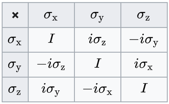
\[\sum_i a_i \sigma_i\]is guaranteed to be Hermitian. Note that the \(\sigma_i\) are not mutually orthogonal in the same sense as mutually orthogonal vectors. Namely,
\[\sigma_i \sigma_j \neq \delta_{ij} I\]Instead, their pairwise products are summarized in the following table:
What can we do with these matrices? So far we’ve measured spin along \(x\), \(y\), or \(z\), but these operators allow us to measure it in any direction. This is done by taking the dot product of the Pauli matrices with the unit vector \(\hat{n}\) along which the measurement is taken.
For example, if we measure along \(\hat{n}=(1/\sqrt{2},1/\sqrt{2},0)\), the operator is
\[\frac{1}{\sqrt{2}} \begin{pmatrix} 0 & 1-i \\ 1+i & 0 \\ \end{pmatrix}\]This operator has eigenvalues \(\pm 1\) and eigenvectors
\[\begin{align*} \ket{+n} &= \frac{1}{2}\begin{pmatrix} 1-i \\ \sqrt{2} \end{pmatrix} \\ \ket{-n} &= \frac{1}{2}\begin{pmatrix} -1+i \\ \sqrt{2} \end{pmatrix} \\ \end{align*}\]These eigenvectors can be used to calculate measurement probabilities. For example, if the spin starts in \(\ket{+z}\), the measurement probabilities are
\[P(+1) = \lvert \bk{+n}{+z} \rvert^2 = 1/2 \\ P(-1) = \lvert \bk{-n}{+z} \rvert^2 = 1/2\]These two probabilities are equal because the measurement happens to be taken at 45 degrees.
Sequential Measurement
What happens after a measurement? Looking back at the principles, the particle “collapses to” or becomes “prepared in” the eigenstate of the measurement result.
For example, consider a spin particle with initial state (in the \(z\) basis)
\[\ket{\psi} = \begin{pmatrix} a \\ b \end{pmatrix}\]If \(\sigma_x\) is measured, the outcome probabilities prior to measurement are
\[\begin{align*} P(\sigma_x = +1) &= \lvert\bk{+x}{\psi}\rvert^2 = \frac{1}{2}(1+a^*b+ab^*) \\ P(\sigma_x = -1) &= 1 - P(+1) = \frac{1}{2}(1-a^*b-ab^*) \end{align*}\]After measurement, the state collapses to either \(\ket{+x}\) or \(\ket{-x}\). If \(\sigma_x\) is measured again it’s guaranteed to return the same value. On the other hand, if afterward the spin is measured in a different direction, the outcome probabilities are all \(1/2\), as per the definition of each state. For example, if the first measurement returned \(\sigma_x = +1\) and we measure \(\sigma_z\), then the outcome probabilities are
\[P(\sigma_z = +1) = \lvert\bk{+z}{+x}\rvert^2 = 1/2 \\ P(\sigma_z = -1) = \lvert\bk{-z}{+x}\rvert^2 = 1/2\]Last
States, operators, and principles wrap up the first part of QM. They lay the foundation for modeling more interesting systems — particles, forces, dynamics, and entanglement — which the next posts will cover. To be continued…