Quantum Mechanics Part II: Dynamics & Continuous States
Dynamics
The Time Evolution Operator
Dynamics for vectors, including those in Hilbert space, can generically be modeled as
\[\ket{\Psi(t_2)}=\mathbf{U}(t_2,t_1) \ket{\Psi(t_1)}\]where \(\mathbf{U}\) is a “time evolution operator” that maps states from one time to another. Usually we set \(t_1=0\) and \(t_2=t\) and simply write \(\mathbf{U}(t,0) \rightarrow \mathbf{U}(t)\).
At this point \(\mathbf{U}\) could be anything, but we require one thing of it: that it conserve inner products. Susskind calls this “conservation of information.” It implies that for arbitrary \(t\), \(\bk{\Psi(t)}{\Phi(t)} = \bk{\Psi(0)}{\Phi(0)}\), or
\[\bra{\Psi(0)}\mathbf{U}(t)^{\dagger}\mathbf{U}(t)\ket{\Phi(0)} = \bk{\Psi(0)}{\Phi(0)}\]So \(\mathbf{U}^{\dagger}\mathbf{U} = I\) and therefore \(\mathbf{U}\) is unitary. A corollary to this is that the magnitude of state vectors is conserved over time.
These results are for finite evolutions. What about infinitesimal ones? To leading order in a small time interval \(\epsilon\), the linear approximation of \(\mathbf{U}\) is
\[\mathbf{U}(\epsilon) = I - \frac{i}{\hbar}\epsilon \mathbf{H}\]where \(\mathbf{H}\) is a constant operator. The factors of \(i\) and \(\hbar\) are conventional: \(i\) ensures that \(\mathbf{H}\) comes out Hermitian under the unitarity requirement (as we verify below), and \(\hbar \approx 10^{-34}\,\text{kg}\,\text{m}^2/\text{s}\) gives \(\mathbf{H}\) units of energy. What does this operator do to \(\ket{\Psi}\)?
\[\begin{align*} \ket{\Psi(\epsilon)} &= \mathbf{U}(\epsilon) \ket{\Psi(0)} \\ \ket{\Psi(\epsilon)} &= \left(I - \tfrac{i}{\hbar}\epsilon \mathbf{H}\right) \ket{\Psi(0)} \\ \frac{\ket{\Psi(\epsilon)} - \ket{\Psi(0)}}{\epsilon} &= -\tfrac{i}{\hbar}\mathbf{H} \ket{\Psi(0)} \\ \end{align*}\]As \(\epsilon \rightarrow 0\),
\[i \hbar \frac{\partial \ket{\Psi}}{\partial t} = \mathbf{H}\ket{\Psi}\]This PDE is called the generalized Schrodinger equation.
Before moving on to solve the GSE, we can learn a bit about \(\mathbf{H}\) by asking what, if anything, the unitary condition on \(\mathbf{U}\) implies about it:
\[\begin{align*} \mathbf{U}(\epsilon)^\dagger \mathbf{U}(\epsilon) &= \left(I - \tfrac{i}{\hbar}\epsilon \mathbf{H}\right)^\dagger \left(I - \tfrac{i}{\hbar}\epsilon \mathbf{H}\right) \\ &= \left(I + \tfrac{i}{\hbar}\epsilon \mathbf{H}^\dagger\right) \left(I - \tfrac{i}{\hbar}\epsilon \mathbf{H}\right) \\ &= I - \tfrac{i}{\hbar}\epsilon \mathbf{H} + \tfrac{i}{\hbar}\epsilon \mathbf{H}^\dagger = I \\ \end{align*}\]So unitarity of \(\mathbf{U}\) implies \(\mathbf{H}\) is Hermitian, and therefore \(\mathbf{H}\) represents an observable. As we’ll see, that observable is the quantum Hamiltonian.
In CM recall that Hamiltonians represent the total energy of a system and relate to the system’s dynamics through the Poisson bracket:
\[\dot{L}=\{L,H\}\]\(L\) here is any quantity defined over phase space \(L(q,p)\). Using the GSE it’s straightforward to show that a similar relation exists in QM but for expected values (assuming \(\mathbf{L}\) has no explicit time dependence, which is true for most observables we care about):
\[i \hbar \frac{d}{dt}\left<\mathbf{L}\right> = \left<\left[\mathbf{L},\mathbf{H}\right]\right>\]\(\left[\mathbf{L},\mathbf{H}\right] = \mathbf{L}\mathbf{H} - \mathbf{H}\mathbf{L}\) is called the commutator. From it we see that if a quantity commutes with \(\mathbf{H}\) then it’s conserved (in expectation), and more generally any function of a quantity that commutes with \(\mathbf{H}\) is conserved (in expectation). This is like in CM where if the PB is \(0\) then \(L\) is conserved.
In QM, expected values don’t change because the measurable outcomes change—those are fixed by the operator (e.g., \(\pm 1\) for spin). They change because the probabilities of each outcome change, and computing how they change requires solving the generalized Schrodinger equation.
Solving the Generalized Schrodinger Equation
Solving the GSE is easiest in the energy basis where \(\mathbf{H}\) is diagonal and an arbitrary state vector can be written as
\[\ket{\Psi(t)} = \sum_i a_i(t) \ket{E_i}\]\(\ket{E_i}\) is an energy eigenvector satisfying \(\mathbf{H}\ket{E_i} = E_i\ket{E_i}\). Inserting this into the GSE gives
\[\begin{align*} \sum_i \dot{a}_i(t) \ket{E_i} &= -\frac{i}{\hbar} \mathbf{H} \sum_i a_i(t) \ket{E_i} \\ &= -\frac{i}{\hbar} \sum_i E_i a_i(t) \ket{E_i}\\ \end{align*}\]This is a simple first-order ODE for each component. The solution is
\[a_i(t) = a_i(0) e^{-iE_it/\hbar}\]Compared to the general form of an oscillator \(\exp(-i \omega t)\) we see that \(E/\hbar\) plays the role of frequency in QM.
This solution assumes we’re working in the energy basis. What if we’re given a state vector in another basis—say the spin basis \(\ket{+z}, \ket{-z}\)? Diagonalize the Hamiltonian as \(\mathbf{H} = \mathbf{P}\mathbf{\Lambda}\mathbf{P}^{\dagger}\); the state in the energy basis is then \(\mathbf{P}^{\dagger}\ket{\Psi}\), with components \(a_i = \bk{E_i}{\Psi}\). Putting it all together, the general solution to the SE is
\[\ket{\Psi(t)} = \sum_i \bk{E_i}{\Psi(0)} e^{-iE_it/\hbar} \ket{E_i}\]Continuous States
Making the Transition
So far we’ve looked at what I’m going to call discrete states—discrete in the sense that eigenvalues are countable and states are written as a finite sum over basis vectors. But we’d also like to model continuous quantities, like position and momentum. How are continuous states modeled?
The answer is that they’re modeled in the same way as discrete states: by the principles of QM. The trick is to keep in mind that the principles don’t require states to be discrete—they only require them to be vectors, and vectors can be anything, discrete or continuous, as long as they satisfy the axioms of a vector space (closure under addition and scalar multiplication, commutativity and associativity of addition, an additive identity and inverse, etc). Complex functions in this sense are continuous vectors and they’re exactly what are used to model continuous states.
Wave Functions
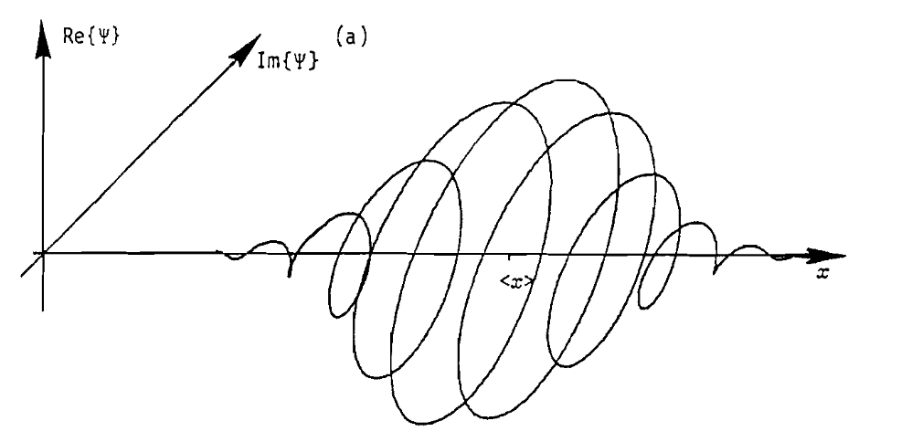
In terms of notation, a continuous state is associated with a wave function \(\psi(x)\) which takes a complex input and returns a complex output. Wave functions are defined with respect to a basis just as discrete vectors are, and their values can change from one basis to another, just as discrete vectors can. The bra-ket notation is useful for wave-functions like it is for discrete vectors. The discrete representation
\[\ket{A} = \sum_i a_i \ket{i}\]becomes
\[\ket{\Psi} = \int \psi(x) \ket{x} \,dx\]where \(x\) labels eigenvalues and \(\ket{x}\) is the associated eigenvector. In the analogy with discrete states, \(\psi(x)\) is like a continuous set of coefficients \(a_i\). Another way to think of wave functions is in terms of a state vector’s projection onto a basis. For example, in the \(x\) basis the wave function is
\[\psi(x) = \bk{x}{\Psi}\]| The probability of measuring a continuous eigenvalue is analogous to the discrete case—it’s \(\psi^*(x)\psi(x)\), the probability density for the random variable \(x\). Because this is a density, the probability of measuring any single value is zero; we should instead talk about the probability of measuring a value in a small region \(dx\) around \(x\), which is $$ | \psi(x) | ^2\,dx$$. |
Continuous Operators
Operators on continuous vectors are similar to operators on discrete vectors: they’re linear and Hermitian. To verify linearity you check that they distribute over the sum of functions with constants factoring out. In other words, \(\mathbf{L}(a\psi(x)+b\phi(x)) = a\mathbf{L}\psi(x) + b\mathbf{L}\phi(x)\)
Examples of linear operators include multiplication by \(x\) and differentiation by \(d/dx\).
Hermiticity is a bit trickier to verify. It occurs when
\[\bke{\psi}{\mathbf{L}}{\phi} = \bke{\phi}{\mathbf{L}}{\psi}^{*}\]Where
\[\bke{\psi}{\mathbf{L}}{\phi} = \int \psi^*(x)\mathbf{L} \phi(x) \,dx\]For example, if \(\mathbf{L}=x\) this is
\[\begin{align*} \bke{\psi}{x}{\phi} &= \int \psi^*(x) x \phi(x) \,dx \\ &= \left( \int \psi(x) x \phi^*(x) \,dx \right)^* \\ &= \bke{\phi}{x}{\psi}^* \end{align*}\]Therefore the operator \(x\) is Hermitian. The \(*\) above is just complex conjugation of the scalar inner product—the same role it plays in the discrete case \(\bke{\psi}{\mathbf{L}}{\phi} = \bke{\phi}{\mathbf{L}}{\psi}^*\). The adjoint \(\mathbf{L}^\dagger\) of a continuous operator is still well-defined; for a differential operator it’s computed via integration by parts rather than a matrix transpose. Applying the Hermiticity test to \(d/dx\) we find that it’s not Hermitian (integration by parts produces a minus sign), but if we multiply it by \(i\) it is.
Position & Momentum
How are eigenvalues and eigenvectors computed for continuous operators? For position the operator is \(x\) and its eigenvalues are denoted by \(x_0\). The eigenequation is
\[x\psi(x) = x_0 \psi(x)\]or
\[(x-x_0)\psi(x) = 0\]If \(x \ne x_0\) then this requires \(\psi(x) = 0\), and when \(x = x_0\) then \(\psi(x)\) can be anything. Up to a scalar, the unique distribution satisfying this equation is the Dirac delta, so the eigenfunction is
\[\psi(x) = \delta(x-x_0)\]| This states the obvious fact that if a particle is measured at \(x_0\) then it’s only at \(x_0\). Note that \(\delta(x-x_0)\) is not square-integrable, so position eigenstates can’t be normalized in the usual sense $$\int | \psi | ^2\,dx = 1\(. Instead they're normalized in the distributional sense\)\bk{x’}{x} = \delta(x-x’)\(, which is consistent with treating\)\delta$$ as a distribution that belongs inside an integral: |
It’s also important to note that this delta-function model of position is a mathematical idealization. If wavefunctions did in fact collapse to delta-functions when position was measured, the uncertainty in position would be zero and, because of the position-momentum uncertainty relation, this would force momentum uncertainty to be infinity, which isn’t physically meaningful.
What are the eigenfunctions of momentum? The set-up and solution are the same, except we now write \(\bar\psi\) for a wave function in momentum space:
\[p\bar\psi(p) = p_0\bar\psi(p) \\ \rightarrow \bar\psi(p) = \delta(p-p_0)\]The \(\delta\) function solution here and for position are not especially insightful, but when we look at momentum in the \(x\) basis things are more interesting. In the \(x\) basis, from experimental insight, the momentum operator changes from \(p\) to \(-i\hbar \, d/dx\). The eigenequation becomes
\[-i\hbar \frac{d}{dx}\psi(x) = p \psi(x)\]and the solution is
\[\psi(x) = Ae^{ipx/\hbar}\]Note that because this is a wavefunction in the \(x\)-basis it’s considered a function of \(x\) and not \(p\). The \(p\) appears because each value of momentum has a different wavefunction associated with it, so \(p\) acts more like a parameter or index.
The constant \(A\) is determined by normalization:
\[\bk{\psi}{\psi} = \int_{-\infty}^{\infty} \psi(x)^*\psi(x) \,dx = 1\]But this gives
\[|A|^2\int_{-\infty}^{\infty} \,dx = 1\]Which is undefined. This reflects the fact that plane-wave momentum eigenstates aren’t physical states on their own—they’re idealized basis functions. Physical states are wave packets, superpositions of plane waves over a range of momenta, which decay at infinity and so are square-integrable. Bound states in a potential well are normalizable for the same reason.
Changing Basis
Generally speaking, a state vector \(\ket{\Psi}\) can be represented in any basis. For example, in the \(x\) basis \(\psi(x) = \bk{x}{\Psi}\), in the momentum basis \(\bar\psi(p) = \bk{p}{\Psi}\), etc. Because these representations ultimately correspond to the same state, namely \(\ket{\Psi}\), there must be a way to transform between them. How do we transform between the \(x\) and \(p\) basis?
The trick is to use the identity operator:
\[I = \int \ket{x}\bra{x} \cdot \,dx\]Where “\(\cdot\)” is a placeholder for the vector which the operator acts on. Inserting this into the momentum-representation gives
\[\begin{align*} \bar\psi(p) &= \bk{p}{\Psi} \\ &= \bke{p}{I}{\Psi} \\ &= \int \bk{p}{x}\bk{x}{\Psi}\,dx \\ \end{align*}\]But
\[\begin{align*} \bk{p}{x} &= \int A e^{-ipx'/\hbar} \delta(x'-x) \,dx' \\ &= Ae^{-ipx/\hbar} \end{align*}\]And \(\bk{x}{\Psi} = \psi(x)\), so
\[\bar\psi(p) = A\int e^{-ipx/\hbar} \psi(x) \, dx\]Which is the formula for converting a position-space wave function into its momentum-space complement. The derivation of the inverse operation is similar. The result is
\[\psi(x) = A \int e^{ipx/\hbar} \bar\psi(p) \,dp\]So position and momentum space are related by the Fourier transform. This leads to the interpretation that momentum space is the spatial frequency domain of position space, where spatial frequency is given by \(k=p/\hbar\).
How do operators change basis? Operators change basis like matrices do: \(\mathbf{L'} = \mathbf{U} \mathbf{L} \mathbf{U}^{-1}\), where \(\mathbf{L}\) is the operator of interest, \(\mathbf{L}'\) is the transformed operator, and \(\mathbf{U}\) is a unitary change-of-basis operator. Because \(\mathbf{U}\) is unitary, \(\mathbf{U}^{-1} = \mathbf{U}^\dagger\).
How does this work for position and momentum? The relevant change-of-basis operator is the Fourier transform \(\mathbf{F}\). Is it unitary? Yes, because \(\mathbf{F}^\dagger\mathbf{F}\psi(x) = \psi(x)\), which implies that \(\mathbf{F}^\dagger\mathbf{F}=I\). Let’s use \(\mathbf{F}\) to derive the position operator in momentum space, call it \(\mathbf{\bar X}\).
\[\begin{align*} \mathbf{\bar X} \bar\psi(p) &= \mathbf{F}\mathbf{X}\mathbf{F}^\dagger \bar \psi(p) \\ &= \mathbf{F} \mathbf{X} \psi(x) \\ &= \mathbf{F} x \psi(x) \\ &= i\hbar \frac{d}{dp} \bar \psi(p) \end{align*}\]Where the last step comes from a Fourier transform identity. So the position operator in momentum space mirrors the form of the momentum operator in position space, but with the opposite sign: \(\mathbf{X} \to +i\hbar\,d/dp\) versus \(\mathbf{P} \to -i\hbar\,d/dx\). That sign asymmetry has physical content—it’s what keeps \([\mathbf{X},\mathbf{P}]\) equal to \(+i\hbar\) in both bases rather than flipping sign.
Another way to determine or verify an operator in a new basis is via commutators, which are basis-independent: e.g., \([\mathbf{X}, \mathbf{P}] = [\mathbf{\bar X}, \mathbf{\bar P}] = i\hbar\). This may require some guess-and-check, whereas the unitary method is explicit and always works—though it can be harder to carry out by hand.
As a practical note, when working with operators it’s helpful to supply them with a test function to act on, otherwise it isn’t always clear exactly how they simplify.
Uncertainty
Going back to the discussion of commutators, we found that two observables are simultaneously knowable iff their operators commute. Do the operators for \(x\) and \(p\) commute? The answer is no. Given \(\mathbf{X}=x\) and \(\mathbf{P}=-i\hbar d/dx\) the commutator is
\[[\mathbf{X}, \mathbf{P}] = i\hbar\]Which means position and momentum aren’t simultaneously knowable—measuring one destroys information about the other, and vice versa. They are said to be incompatible. Just how incompatible? Defining incompatibility in terms of the standard deviation \(\sigma\) of an operator we find from the general uncertainty principle that
\[\sigma_x \sigma_p \ge \frac{\hbar}{2}\]The lower limit on simultaneous uncertainty is reached when \(\psi\) is a Gaussian (equivalently, when \(\bar \psi\) is, since the Fourier transform of a Gaussian is a Gaussian).
What happened to y and z? For the sake of simplicity I’ve focused on measurements taken in one dimension, namely \(x\), but generalizing to \(y\) and \(z\) is straightforward. The position operator for \(y\) is \(y\) and the momentum operator for \(y\) is \(-i\hbar\, \partial/\partial y\). And the same applies to \(z\). Just note that the derivatives change from totals to partials, and the momentum operator as a whole becomes \(-i\hbar \nabla\).
Are measurements compatible across dimensions? The answer is yes. Using \(i\) and \(j\) to index spatial dimensions we get
\[\begin{align*} [\mathbf{X}_i, \mathbf{X}_j] &= 0 \\ [\mathbf{P}_i, \mathbf{P}_j] &= 0 \\ [\mathbf{X}_i, \mathbf{P}_j] &= i\hbar \delta_{ij} \\ \end{align*}\]The Classical Connection
In CM momentum is mass times velocity, while in QM momentum is an observable represented by a Hermitian operator. How are these two pictures related, and is there a general bridge from CM to QM?
The closest we come to a classical-quantum connection is through expected values. For example, in QM the classical notion of velocity corresponds to
\[v \leftrightarrow \frac{d}{dt} \left< \mathbf{X} \right>\]To see why, start by looking at the time-derivative in terms of the Hamiltonian commutator:
\[\frac{d}{dt}\left<\mathbf{X}\right> = -\frac{i}{\hbar}\left<\left[\mathbf{X},\mathbf{H}\right]\right>\]Because \(\mathbf{X}\) commutes with any function of \(\mathbf{X}\), the potential drops out of \([\mathbf{X},\mathbf{H}]\) entirely, and the right side simplifies to \(\left< \mathbf{P} \right>/m\) regardless of whether a potential is present. This is the classical result for velocity. It’s interesting that, unlike in CM, velocity doesn’t appear as a fundamental quantity in QM—momentum takes its place.
What about when a potential is present? In CM the dynamics are
\[\frac{dp}{dt} = -\frac{dV}{dx}\]In QM the left side becomes
\[\frac{d}{dt}\left<\mathbf{P}\right> = -\frac{i}{\hbar}\left<[\mathbf{P},\mathbf{H}]\right>\]The Hamiltonian is
\[\mathbf{H} = \frac{\mathbf{P}^2}{2m} + \mathbf{V}(x)\]Which leads to
\[\frac{d}{dt}\left<\mathbf{P}\right> = -\left<\frac{dV}{dx}\right>\]The quantum result mirrors the classical one in expectation, but with a subtle difference: on the right we take the expectation of the derivative, which is generally not the same as evaluating the derivative at \(\left<x\right>\):
\[\left<\frac{dV}{dx}\right> \neq \frac{dV}{dx} \bigg|_{x=\left<x\right>}\]If the right-hand side held, we could think of a particle as classically “being” at \(\left<x\right>\) and moving according to the potential there, just like a classical particle does, but this isn’t the case. In QM, wavefunctions are spread out in space and therefore “feel” potentials as a distribution—the entire potential function needs to be considered. If, however, the force \(dV/dx\) is approximately constant across the width of the wavefunction—or equivalently, if the wavefunction is narrow compared to the scale on which \(dV/dx\) varies—then the \(\neq\) can be replaced by \(=\), which is the classical limit. Taylor expanding \(V'(x)\) around \(\left<x\right>\) shows the leading correction is \(\tfrac{1}{2}V'''(\left<x\right>)\sigma_x^2\), so the classical equality is exact whenever \(V\) is at most quadratic.
Last
This ends the summary of dynamics & continuous states in quantum mechanics. The framework laid here provides a basis for modeling realistic systems such as free particles, spatially constrained particles, harmonic oscillators, and hydrogen atoms, all of which are covered in the next section. To be continued…