Quantum Mechanics Part 3: Examples
1. The Free Particle
Presumably the simples particle to model is one without any forces acting on it. This is the so-called free particle, its Hamiltonian is
\[\mathbf{H} = \frac{\mathbf{P}^2}{2m} = -\frac{\hbar^2}{2m}\frac{\partial^2}{\partial x^2}\]Note that mass is treated like a fixed parameter instead of an operator like position or momentum. The reason is that mass doesn’t have measurement uncertainty associated with it, it behaves like charge in the sense that it’s intrinsic to the particle and independent of measurement.
Plugging \(\mathbf{H}\) into the GSE yields
\[i\hbar\frac{\partial \psi(x,t)}{\partial t} = -\frac{\hbar^2}{2m} \frac{\partial^2 \psi(x,t)}{\partial x^2}\]This has the form of a diffusion equation but with a complex coefficient, which we’ll see gives rise to wave-like solutions that spread out over time.
The PDE is solved using separation of variables, where the solution is assumed to have the form \(\psi(x,t) = X(x)T(t)\) Plugging this into the PDE and separating \(t\) from \(x\) yields two ODEs, one for each variable, along with a separation constant. The separation constant turns out to be \(E\), and the resulting ODE solutions, when multiplied together produces the overall solution, which can be written several ways:
\[\begin{align*} \psi(x,t) &= \left(Ae^{ix\sqrt{2mE}/\hbar} + Be^{-ix\sqrt{2mE}/\hbar}\right) e^{-iEt/\hbar} \\ &= Ae^{i\left(k x - \omega t\right)} + Be^{-i\left(k x + \omega t\right)} \\ &= \left(A\cos\left(kx\right) + B\sin\left(kx\right)\right) e^{-i\omega t} \end{align*}\]where \(A\) and \(B\) are constants chosen to fit the initial and/or boundary conditions. The wave parameters are \(k = p/\hbar = \sqrt{2mE}/\hbar\) and \(\omega = E/\hbar\).
By inspection, the solution is two planewaves moving in opposite directions and oscillating together at frequency \(\omega\). The phase velocity is
\[v = \omega/k = E/p = p/2m =\hbar k/2m\]The dispersion relation is
\[\omega (k) = \frac{\hbar k^2}{2m}\]In terms of normalization, the wavefunction only normalizes when the particle is bound by a potential. For example, if the particle is un-bound such that it can exist freely in \((-\infty,\infty)\), there’s no way to set \(A\) and \(B\) such that \(\int\psi^*\psi = 1\). Thus, to be physically meaningful, particles must be bound.
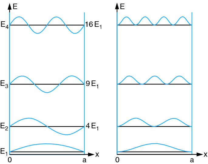
Particle in a box. An example of a bound free particle is the so-called particle in a box. Consider the potential
\[V(0\le x \le L) = 0 \\ V(x < 0) = V(x>L) = \infty\]| This is the so-called “potential well” because it bounds the particle between \(0\) and \(L\). The boundary conditions imply $$ | \psi(0) | ^2 = | \psi(L) | ^2=0$$. Enforcing the boundary condition and normalization yields the solution |
where \(n\in \{1,2,...\}\).
The first few wavefunctions at \(t=0\) are shown below on the left with their probability densities on the right. Interestingly, the boundary conditions force solutions to be countable and have discrete energy levels.
Because the Schrodinger equation is linear any linear combination of the \(\psi_n\) is a solution, so the general solution is
\[\sum_n a_n (0) \psi_n\]where \(a_n(0)\) is the “amount” of \(\psi_n\) in the initial condition, subject to the constraint
\[\sum_n a_n^*(0)a_n(0) = 1\]Because the \(\psi_n\) are an orthogonal set of functions, they can be summed to create an arbitrary wavefunction (up to the boundary conditions) within the well.
Stationary states. Eigenfunctions are sometimes called stationary states. “Stationary” because their PDFs are time-independent. For example, if \(\psi_E(x)\) is an eigenfunction of \(\mathbf{H}\), the wavefunction at time \(t\) is
\[\psi_E(x)e^{-iEt/\hbar}\]which depends on time, but the PDF doesn’t. Note however that the superposition of stationary states isn’t stationary. For example, if \(\psi_1\) and \(\psi_2\) are stationary and normalized individually, then the superposition
\[a\psi_1(x) e^{i\omega_1t} + b\psi_2(x) e^{i\omega_2t}\]has PDF
\[\left| a\psi_1 \right|^2 + \left| b\psi_2 \right|^2 + a^*b\psi_1^*\psi_2\cos((\omega_1-\omega_2)t) + ab^*\psi_1\psi_2^*\sin((\omega_1-\omega_2)t)\]which depends on time. But keep in mind that if the energy of the system is measured it returns just one of the eigenvalues \(E_1\) or \(E_2\) (corresponding to \(\omega_1\) and \(\omega_2\)) and the wavefunction collapses to the corresponding stationary state.
The Gaussian Wavepacket. The Gaussian wavepacket is a common wavefunction used to model unbound free particles. The wavefunction has Gaussian shape so its density is Normally distributed, which makes it ideal for modeling localized particles.
It may seem like Gaussian wavepackets aren’t realizable because unbound wavefunctions don’t normalize, and that’s true—if an unbound free particle has a single definite energy then the wavefunction doesn’t normalize. However, linear combinations of wavefunctions weighted properly over many different energies can normalize, and this is how unbound free particles are constructed mathematically.
So how does this work? Consider the general solution of the SE derived earlier for discrete vectors: \(\ket{\Psi(t)} = \sum_i \bk{E_i}{\Psi(0)} \ket{E_i} e^{-i E_i t/\hbar}\) The continuous version is \(\psi(x,t) = \int \left( \int \psi_E^*(x) \psi(x,0) \,dx \right) \psi_E(x) e^{-iEt/\hbar} \, dp\) Where \(\psi(x,0)\) is an intial condition and the integrals run from \(-\infty\) to \(+\infty\). Normally we have \(\psi_E(x) = Ae^{ik x } + Be^{-ik x}\) but because the integral covers negative and positive values of \(x\) we can just focus on one of the terms without loss of generality. We’ll focus on the first term. The result is \(\begin{align*} \psi(x,t) &= \int \left( \int e^{-ipx/\hbar} \psi(x,0) \,dx \right) e^{-iEt/\hbar} e^{ipx/\hbar} \, dp \\ &= \int \left(\mathbf{F}\psi(x,0)\right) e^{i(kx-\omega t)} dk \\ &=\int \bar\psi(k,0)e^{i(kx-\omega t)}dk \end{align*}\) So the general solution is a sum of planewaves weighted by the “amount” of each wave present in the initial condition. Because each planewave moves at a different speed—its phase speed—the initial waveform spreads out over time.
To make a Gaussian wavepacket, consider the following initial condition in momentum-space:
\[\bar\psi(p,0) = \frac{1}{(2\pi \sigma_p^2)^{1/4}} \exp (-\frac{(p-p_0)^2}{4\sigma_p^2})\]When squared this wavepacket is Gaussian centered at \(p_0\) with spread \(\sigma_p\). In position space this wavefunction is
\[\psi(x,0) = \left( \frac{4 \sigma_p^2 \hbar^2}{2\pi} \right)^{1/4} \exp(-\sigma_p^2 x^2 /\hbar^2) \exp(ip_0x/\hbar)\]Which is a Gaussian multiplied by a wave factor. By inspection, the position space uncertainty is related to the momentum space uncertainty by \(\sigma_x \sigma_p = \hbar/2\), which is exactly the lower limit of the Heisenberg uncertainty relation.
Note that plugging \(\psi(x,0)\) into the SE we find that it’s not a solution.
Plugging \(\bar \psi(p,0)\) into the GSE solution and taking the integral gives
\[\psi(x,t) = \frac{(2\pi\sigma_x^2)^{-1/4}}{\left(1+i\frac{\hbar}{2m\sigma_x^2}\right)^{1/2}}\exp \frac{-x^2+\frac{i}{\hbar}(4\sigma_x p_0 x + 2\sigma_x^2p_0^2t)}{4\sigma_x^2(1+i\frac{\hbar}{2m\sigma_x^2}t)}\]This is a complicated looking wavefunction, but its density is a Gaussian:
\[\lvert \psi(x,t) \rvert^2 = \frac{1}{\sqrt{2\pi\sigma_x^2(t)}} \exp -\frac{\left( x-\mu(t) \right)^2}{2\sigma^2_x(t)}\]Where
\[\begin{align*} \mu(t) &= \frac{p_0}{m}t \\ \sigma_x(t) &= \sigma_x \sqrt{1+\left(\frac{\hbar}{2m\sigma_x^2}t\right)^2} \end{align*}\]So the center of the wavepacket moves with group velocity \(p_0/m\) just like a classical particle, and the phase waves disperse causing the packet to spread over time. The spread increases like \(\sqrt{1+t^2}\), so the particle becomes less localized and the product \(\sigma_x\sigma_p\) rises above the Heisenberg lower limit.
What happens when a Gaussian wavepacket is measured? If its energy is measured to be, say, \(E_0\) then the wavefunction collapses to the eigenfunction corresponding to that energy, namely \(\exp(ix\sqrt{2mE_0}/\hbar)\).
2. Harmonic Oscillator
The quantum harmonic oscillator is modeled with a quadratic potential just like its classical counterpart. The Hamiltonian is
\[\mathbf{H} = \frac{\mathbf{P}^2}{2m} + \frac{1}{2}m\omega^2\mathbf{X}^2 = -\frac{\hbar^2}{2m}\frac{\partial^2}{\partial x^2} + \frac{1}{2}m\omega^2x^2\]where \(\omega\) is the oscillator’s frequency parameter (not to be confused with phase frequency). Plugging this into the GSE gives
\[i\frac{\partial \psi}{\partial t} = -\frac{\hbar}{2m} \frac{\partial^2 \psi}{\partial x^2} + \frac{m \omega^2}{2\hbar}x^2\psi\]As usual, the approach is to find the energy eigenfunctions, then multiply them by the time-dependent factor \(\exp(-iE_it/\hbar)\) and sum the eigenfunctions to make a general solution.
The energy eigenequation (also called the time-independent schrodinger equation TISE) is
\[-\frac{\hbar^2}{2m}\frac{d^2 \psi_E}{d x^2} + \frac{1}{2} m \omega^2 x^2 \psi_E = E\psi_E\]This equation turns out to have solutions for every value of \(E\) (including complex \(E\)), but only a few solutions normalize as is required for the wavefunction to be physically meaningful. The result is that for each \(n \ge 0\) the \(n\)th normalizable energy is
\[E_n = n\hbar\omega + \frac{\hbar\omega}{2}\]and the wavefunction is
\[\psi_n(x) = \sqrt{\frac{a}{2^n n! \sqrt{\pi}}} H_n(ax) e^{-a^2x^2/2}\]where \(a = \sqrt{\omega m / \hbar}\) and \(H_n\) are Hermite polynomials. The probability densities of the first few energies are shown below along with the quadratic oscillator potential.
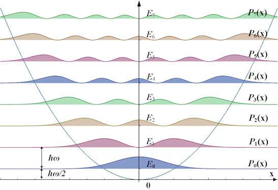
There are a few interesting things to notice…
- The minimum energy is not zero—it’s \(\hbar \omega /2\). So for an oscillator to exist at all some energy is required. This can be understood in terms of the uncertainty principle: suppose we try to make the total energy zero by closely localizing the particle to \(x=0\). In this case the potential energy will be approximately zero, but the momentum will be very spread out, and momentum has energy associated with it. On the other hand if we try to set the particle at rest so it has no momentum then the position will be spread out, in particular it will be spread out away from \(x=0\) and therefore have potential energy. So either way the oscillator has some energy.
- Energy levels don’t depend on mass (in constrast to particle in a box).
- Hermite polynomials are orthogonal (they better be—they’re eigenvectors).
- Probability densities are non-zero outside the potential energy curve, so the particle can be found beyond the classically allowed region.
- Inside the classically allowed region there are points where the density is zero, so the particle will never be measured there even though it can be classically.
- In the limit of large \(n\) the quantum density approaches the classical density.
- Succesive energy levels add one “bump” to the probability density.
4. Tunnelling
5. The Spherical Equation
When it’s natural to describe a quantum system in terms of sperical coordinates we can use \(r,\theta,\phi\) instead of \(x,y,z\). For spherical coordinates the physics convention is \(0\le r < \infty \\ 0 \le \theta \le \pi \\ 0 \le \phi \le 2\pi\)
The spherical TISE is \(\left(-\frac{\hbar^2}{2m}\nabla^2 + V(r)\right)\psi(r,\theta,\phi) = E\psi(r,\theta,\phi)\) where \(V\) is assumed to depend only on \(r\). Note that we don’t need to re-consider the temporal component of the SE when changing coordinates. The reason is that the temporal factor is \(\exp(-iE_i t/\hbar)\), regardless of which spatial coordinates we use. So the time-dependent part is already solved, we just need to solve the spatial part and multiply it by this time factor to get the final wavefunction.
The next step is transforming \(\nabla^2\) into spherical coordinates. The result is \(-\frac{\hbar^2}{2m}\frac{1}{r^2}\left[ \partial_r(r^2\,\partial_r\psi) + \frac{1}{\sin\theta} \, \partial_\theta(\sin\theta\,\partial_\theta\psi) +\frac{1}{\sin^2\theta}\,\partial_\phi^2\psi \right] + V(r)\psi = E\psi\) To solve this PDE we can use separation of variables, where we assume \(\psi(r,\theta,\phi)=R(r)\Theta(\theta)\Phi(\phi)\). This leads to three ODEs, one for each coordinate: \(\Phi''=m^2\Phi \\ k\sin^2\theta-\frac{\sin^2\theta}{\Theta}(\Theta''+\cos\theta\sin\theta\,\Theta')=m^2 \\ \frac{2rR'+r^2R''}{R} +\frac{2m}{\hbar^2}r^2(E-V(r))=k\) Here, \(m\) and \(k\) are constants arising from the variable separation (\(m\) is squared for convenience, the alternative is to not square \(m\) and instead write a square-root everywhere it appears, but square-roots are annoying to draw and look at and I think there’s pretty good consensus on that!).
The solution for \(\Phi\) is sinusoidal, and because it’s periodic \(m\) is forced to be an integer.
The solution for \(\Theta\) is more involved. I’ll just say that it only converges when \(k=l(l+1)\) where \(l \in \{0,1,2,...\}\) and \(m \in \{-l,-l+1,...,l-1,l\}\). So for a given \(l\) there are \(2l+1\) allowed values of \(m\).
Multiplied together, the angular functions are the so-called spherical harmonics \(Y_l^m(\theta,\phi)=\Theta(\theta)\Phi(\phi)\), where \(l\) and \(m\) are quantum numbers. When building a solution, \(l\) is generally chosen before \(m\) because the allowed values of \(m\) depend on which \(l\) is chosen. Spherical harmonics generally arise when the Laplacian is solved in polar coordinates, but they don’t encode any real physics (other than perhaps angular periodicity). Everything physical—mass, energy, Plank’s constant—is in the \(R\) equation. So regardless of the potential we’re working with we can focus on solving the \(R\) ODE and then multiply the solution by \(Y\) to get the overall (spatial) solution.
The \(R\) ODE is simplified by changing variables \(u(r)=rR\). The result is \(\left[-\frac{\hbar^2}{2m}\frac{d}{dr} + \frac{\hbar^2l(l+1)}{2m}\frac{1}{r^2} + V(r) \right]u(r) = Eu(r)\) If we interpret the effective potential as \(V_{\textnormal{eff}} = \frac{\hbar^2l(l+1)}{2m}\frac{1}{r^2} + V(r)\) then the radial equation looks like the Cartesian SE, but with an extra term for angular momentum. Keep in mind that \(u\) must be zero as \(r \rarr 0\), and \(u\) needs to be divided by \(r\) before being interpereted physically.